Bezier Curves
May 8, 2022
Freddy
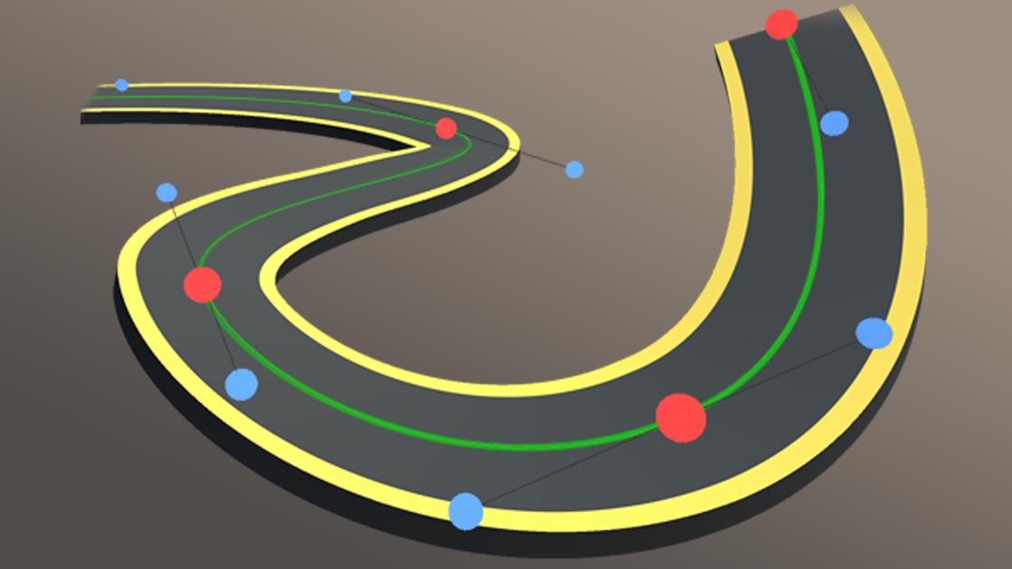
If you’ve ever worked with vector art, you’ve almost certainly come across Bezier curves. But what exactly are they? This article explains how to construct a Bezier curve, discusses where they are used, and describes underlying mathematics.
A Bézier curve is smooth and continuous.
It is not computationally expensive, so it is used in computer graphics (drawing fonts and other vector images). It also has nice properties, for example, its derivatives are easy to compute. Hence, its application extends to robotics and modelling highway design.
What is a Bezier curve?
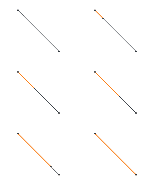
Let’s begin by linear interpolating (lerping) over 2 points. That is, we move from 1 point to the other.
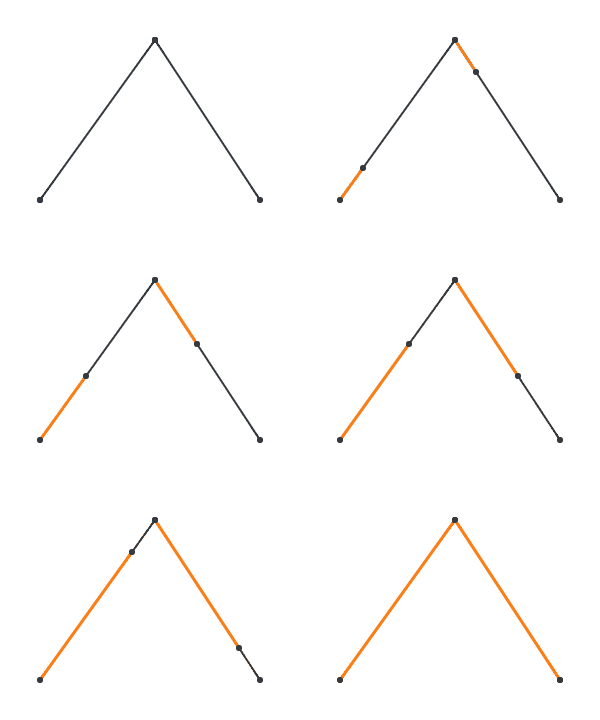
Now, consider 3 points P, Q, R. Lerp over P and Q, and lerp over Q and R. Let’s call the moving points A and B.
Now, lerp over A and B, and we get a curve!
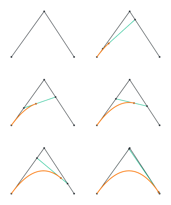
This is the idea behind constructing a Bezier curve. We call P, Q, R our control points. With 3 control points, we have 2 stages of lerping to generate a quadratic Bezier curve. We can add an additional control point, which generates a cubic Bezier curve through 3 stages of lerping.
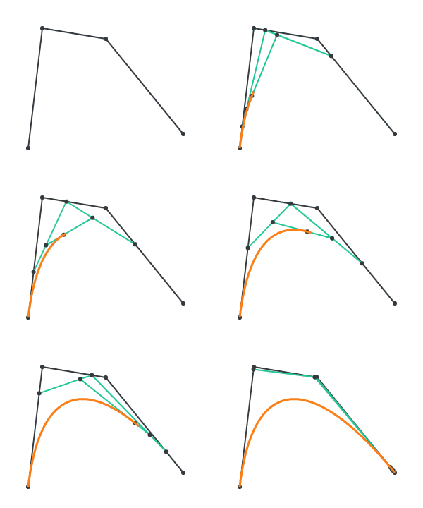
We can keep adding control points indefinitely, although quadratic and cubic Bezier curves are used most often.
By moving the control points, we can form all kinds of curves. Here’s an exotic curve below.
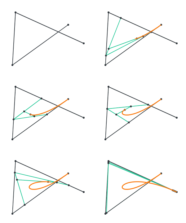
We can generate further shapes by joining multiple Bezier curves together to form B-splines. We will explore this later.
Try it out yourself!
Drag the control points with your mouse.
Bezier curves in vector art
Here is a path I drew in Inkscape, a vector editor.
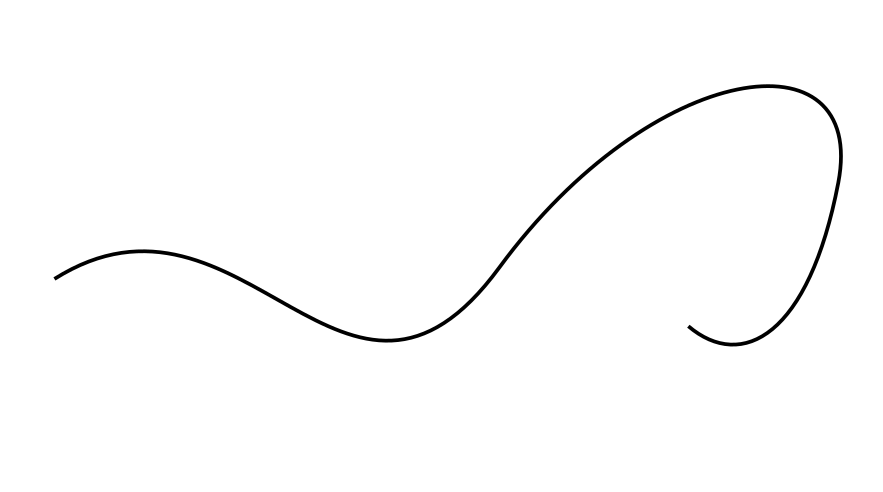
Selecting the path reveals some details.
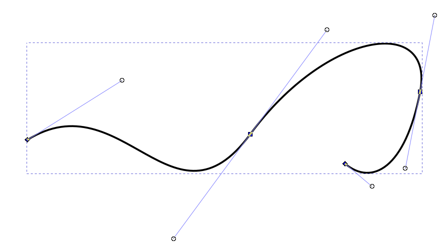
These details reveal that the path is, in fact, 3 cubic Bezier curves fused together. We annotate one curve below.
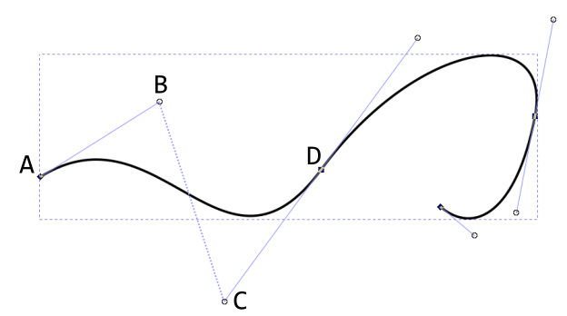
Recall how Bezier curves are lightweight: they are defined very easily. In fact,
this is how the path is defined (in the .svg file).
<path
  d="m 30.980769,120.80769 c 20.076924,-12.63461 30.980768,20.94231 47.25,
     -1.21154 16.269229,-22.153843 39.115381,-25.269227 36.000001,-9 -3.11539,
     16.26923 -10.21154,20.07693 -15.92308,15.23077"
  id="path1901"
/>
A quick count yields 10 pairs of coordinates. This makes sense, as we expect 12 control points for 3 cubic Bezier curves, but 2 points are shared.
The maths behind Bezier curves
De Casteljau’s algorithm
Recall how we constructed Bezier curves through recursive lerping. To lerp between 2 points \(p\) and \(q\), we use this equation:
\[(1 - t)p + tq \quad t \in [0, 1]\]Let \({p_0, \ldots, p_n}\) be the control points. Define the following recurrence relation.
\[\begin{align} &p_i^{(0)}(t) = p_i & &i = 0, \ldots, n\\ &p_i^{(j)}(t) = (1 - t)p_i^{(j-1)} + t p_{i+1}^{(j-1)} & &i = 0, \ldots, n-j \end{align}\]Intuitively, \(p_i^{(j)}(t)\) describes the intermediary lerped points at time \(t\). The actual point along the Bezier curve at time \(t\) is \(p_0^{(n)}(t)\), which we denote as \(B(t)\).
Bernstein form
By expanding the recurrence relation in De Casteljau’s algorithm, we get the explicit representation. This is the Bernstein form.
As a reminder, \({p_0, \ldots, p_n}\) are the control points, and \(B(t)\) is our point along the Bezier curve.
\[\begin{align} &B(t) = \sum_{i=1}^n b_{i, n}(t) p_i & & \\ &b_{i, n}(t) = \binom{n}{i} (1-t)^{n-i} t^i & &\text{(Bernstein basis polynomials)} \end{align}\]In this form, it is easy to compute the derivative of any point along a Bezier curve. This is useful in applied mechanics, for example, when the vertical heights of roads or other platforms are modelled as Bezier curves.
\[B'(t) = n \sum_{i=0}^{n-1} b_{i, n-1}(t) (p_{i+1} - p_i)\]Further reading
- On a separate blog post, I give a tutorial on how to write a program that draws Bezier curves.
- The Beauty of Bezier Curves is an exceptional, beginner-friendly video that discusses more properties of Bezier curves.
More Blog Posts
The Intuition behind Convolutional Neural Networks
The UCI Protocol for Chess Engines
Setting Up Unrestricted ChatGPT Locally on Mac
Histogram Equalisation for Colour Images
Enhancing Greyscale Image Contrast through Histogram Equalisation
On the Philosophy and Design Choices of this Site
Benchmarking Loops in JavaScript
Looping Through a List in JavaScript