Support Vector Machines

Mar 1, 2023
Freddy

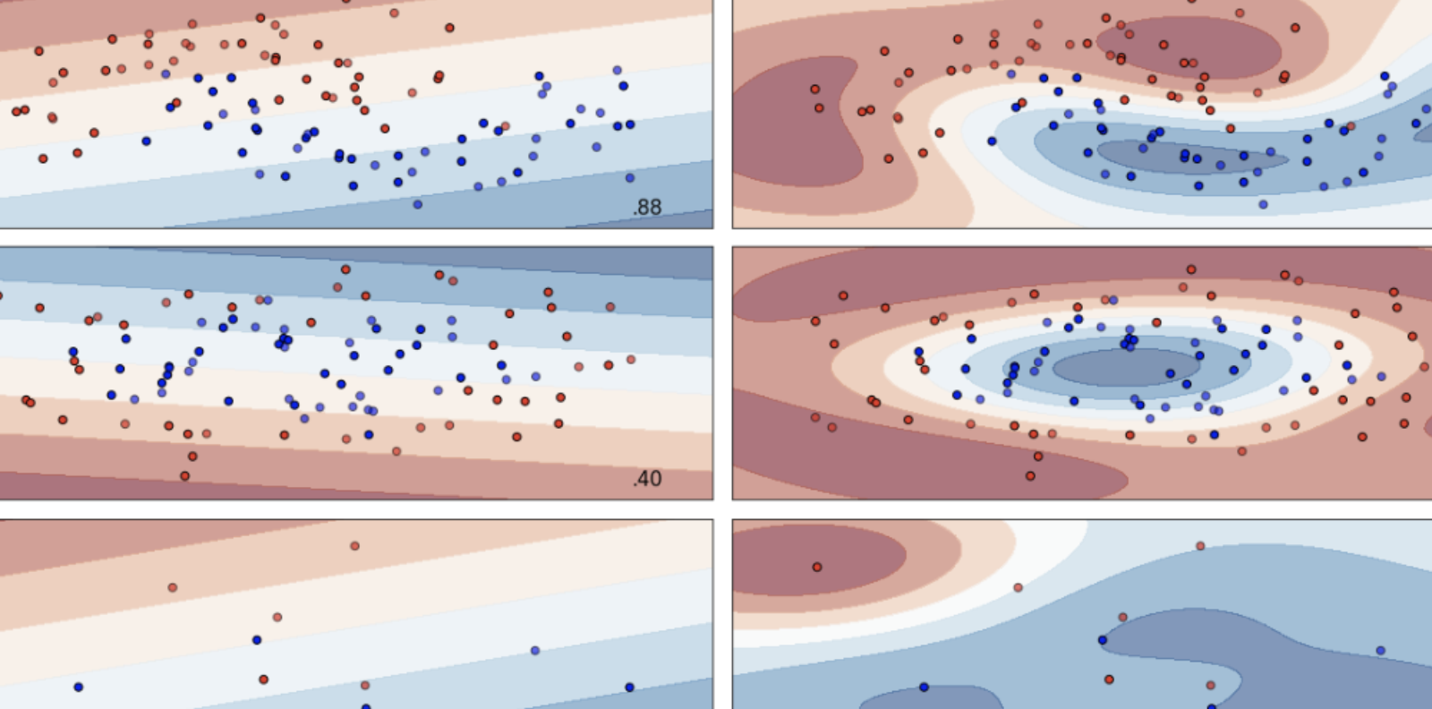
A support vector machine is a powerful and simple machine learning architecture that used to be state-of-the-art in image classification. In this article, we delve into the intricacies of support vector machines and its applications in linear, non-linear, binary and multi-class classification.

Motivation

Say we have two types of fungi in our backyard: honey mushroom and velvet shank. We also have some data points, where each data entry records the type of fungi, as well as its height and cap width. We plot the data points as such.

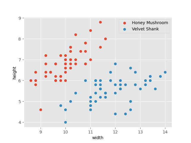
We can empirically observe a relationship between the features of each fungus (i.e. height and cap width) and its type. Let’s draw a line to separate them.

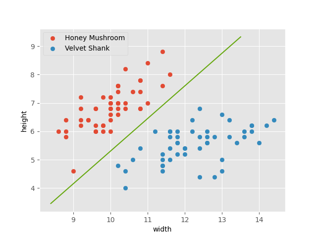
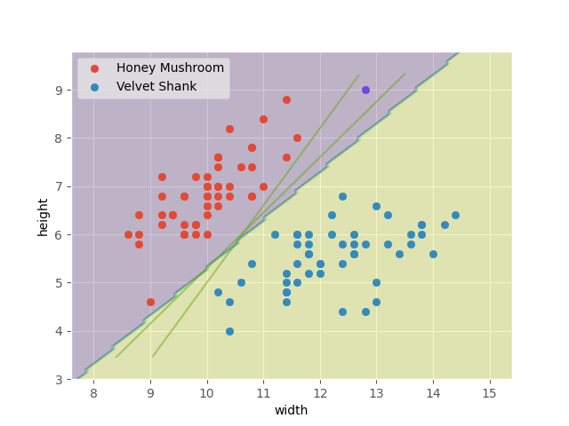
This line describes a very simple model! We can use this line to predict the type of new fungi in our backyard. Say we go measure a mushroom and get a height of 9 and cap width of 12.8.

The model predicts the fungus as a honey mushroom. But what if we draw the line a bit differently? Consider the model below. The line still separates our original data perfectly, but now our model predicts the fungus as a velvet shank.

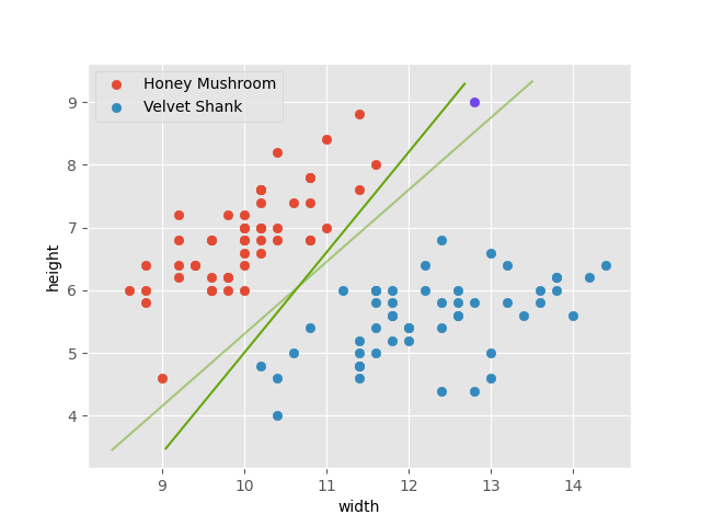
How do we determine the best line?

This leads us to support vector machines (SVMs). An SVM is a very powerful supervised learning method that mathematically formulates the optimal model for binary classification.

Woah! I've thrown in a lot of machine learning terminology already. Let's go through them.

Binary classification refers to the task of categorising input data into one of 2 classes. In our case, the input data is the set of features describing each fungus: height, cap width. Our 2 classes are honey mushroom and velvet shank.

Supervised learning refers to training a model using data points with labels. In our case, we have some initial data points where we already know the type of mushroom. The counterpart is unsupervised learning: we have the set of features (height, cap width) but no corresponding label during training.

SVM is a supervised learning technique. However, unsupervised learning is also very useful! For example, we can train a model to cluster data points into groups, or perform dimensionality reduction.

We will start off with the simplest case: finding the optimal linear model that separates data points into exactly 2 groups. Later, we briefly discuss generalising this to non-linear models that classify points into an arbitrary number of groups.

Binary linear classifier

A hard-margin binary classifier defines a hard linear boundary that perfectly separates the 2 classes. We start by deriving the optimisation problem from scratch.

Warning: This section is maths-heavy. You can skip to "Generalisations and extensions".

Initial steps

Let ${x_1, x_2}$ represent height and cap width. We can define a linear model as:

\[w_1 x_1 + w_2 x_2 + b = 0\]

The optimal line is determined by ${w_1, w_2}$ and $b$. This can be rearranged to slope-intercept form:

\[x_2 = -\frac{w_1}{w_2} x_1 - \frac{b}{w_2}\]

Here, we make an important observation. The gradient of the line is ${ \begin{bmatrix} 1 \\ -\frac{w_1}{w_2} \end{bmatrix} }$. That is, as $x_1$ moves by $1$, $x_2$ moves by ${-\frac{w_1}{w_2}}$. This is analogous to ${y = mx + c}$: as $x$ moves by $1$, $y$ moves by $m$.

Define ${w = \begin{bmatrix} w_1 \\ w_2 \end{bmatrix}}$.

\[\begin{bmatrix} w_1 \\ w_2 \end{bmatrix} \cdot \begin{bmatrix} 1 \\ -\frac{w_1}{w_2} \end{bmatrix} = 0\]

Hence, $w$ is orthogonal to the gradient.

Extending to higher dimensions

We can partition a 2D plane into 2 regions using a 1D line. Similarly, we can partition a 3D space into 2 regions using a 2D plane.

Let $n$ be the number of features. In general, we can partition an $n$-dimensional space using an ${(n-1)}$-dimensional hyperplane.

\[w \cdot x + b = 0\]

Our previous observation still holds: $w$ is orthogonal to the gradient of our hyperplane.

Formulating the problem

We want the maximum margin hyperplane: let ${c_1, c_2}$ be the distance between the hyperplane and the closest points to it from each class. We denote the closest points ${x_1, x_2}$. Hence, the hyperplane should be defined such that it perpendicularly bisects the line segment formed by $c_1$ and $c_2$. Then, ${c_1 = c_2}$. We can always normalise our data, so we generalise ${c_1 = 1}$.

Define our 2 classes as ${\{+1, -1\}}$. Define the binary classifier as follows:

\[c = \begin{cases} +1 & w \cdot x + b \geq 0 \\ -1 & \text{otherwise} \end{cases}\]

Then, our problem is to derive the margin between ${w \cdot x_1 + b = 1}$ and ${w \cdot x_2 + b = -1}$.

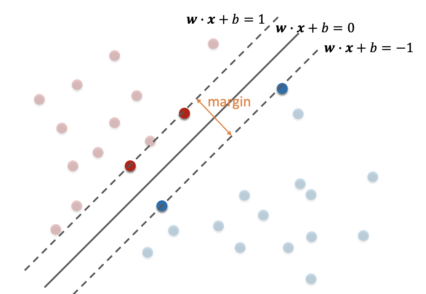
Define the margin size as $m$. Then ${x_2 = x_1 + mn}$, where $n$ is the standard normal to ${w \cdot x_1 + b = 1}$. Now, we have:

\[\begin{align} w \cdot x_1 + b &= 1 \\ w \cdot (x_1 + mn) + b &= -1 \end{align}\]

Subtracting equation 2 from 1 we get:

\[mw \cdot n = 2\]

We now use our previous observation to formulate $n$ as $\frac{w}{\|w\|}$. Hence, ${m = \frac{2}{\|w\|}}$.

A hard-margin binary linear classifier can be described as the following optimisation problem.

\[\begin{align} \max_{w, b} & \frac{2}{\|w\|} \\ \text{subject to} \ & w \cdot x_i + b \geq +1 \quad y_i = +1 \\ & w \cdot x_i + b \leq -1 \quad y_i = -1 \quad \text{for each datapoint ${(x_i, y_i)}$} \end{align}\]

What if there is no such clear-cut line?

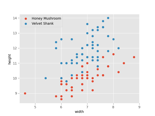
In this case, we allow some training points to be misclassified by no longer enforcing the 2 constraints - instead, we add a penalty term for every misclassified point. This is called a soft-margin classifier and can be reformulated as the Hinge loss:

\[\min_{w, b} L(w, b) = \|w\|^2 + \lambda \sum_{i=1}^N \max{(0, 1 - y_i (w \cdot x_i + b))}\]

where $\lambda$ is a hyperparameter corresponding to penalty strength.

If a point is correctly classified, the penalty term is $0$. Otherwise, the penalty is how badly the point is misclassified, defined by the distance to the line: ${1 - y_i (w \cdot x_i + b)}$.

Training the model: Gradient descent

We formulated a loss function $L$ that we want to minimise. To find optimal values of our parameters $w$ and $b$, we initialise $w$ and $b$ to arbitrary values then use gradient descent to finetune them.

\[\begin{align} w^{(k+1)} &= w^{(k)} - \alpha \triangledown_w L(w^{(k)}, b^{(k)}) \\ b^{(k+1)} &= b^{(k)} - \alpha \triangledown_b L(w^{(k)}, b^{(k)}) \end{align}\]

where ${w^{(k)}, b^{(k)}}$ are the values at iteration $k$ and $\alpha$ is the learning rate.

Our loss function includes the following: $$\sum_{i=1}^N \max{(0, 1 - y_i (w \cdot x_i + b))}$$ N denotes the number of training data samples. If N is very large, it takes lots of time to compute L. Do we have a workaround?

The solution is to use stochastic gradient descent (SGD): instead of using the entire dataset to compute L each iteration, we only use a random subset (mini-batch). This allows us to perform each iteration faster while still working towards the optimal values of w and b. The term now becomes: $$\sum_{i \in M \subset N} \max{(0, 1 - y_i (w \cdot x_i + b))}$$ where M is a different random subset every iteration.

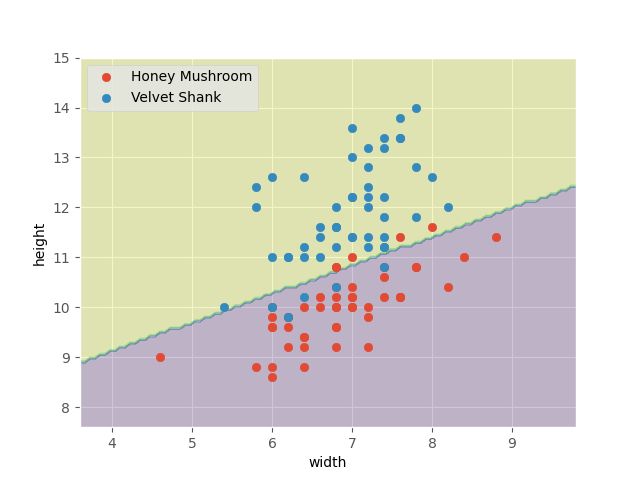
After training, this is our optimal model.

For our soft-margin example, the optimal model is shown below.

Generalisations and extensions

Multi-class classification

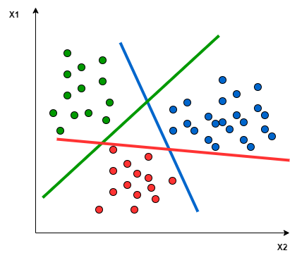
SVMs are intrinsically for binary problems. There are ways to reformulate multi-class problems to be solved with SVM. Let’s assume there are 4 classes: apple, banana, cherry, dates.

One-to-Rest: We decompose the original problem into 4 binary problems: apple vs other classes, banana vs other classes, etc.
One-to-One: We have a binary problem for each pair of classes: apple vs banana, apple vs cherry, banana vs cherry, etc.

Kernel trick

SVMs intrinsically describe linear relationships. The kernel trick applies a kernel that maps data points to a higher dimensional space that may be linearly separable.

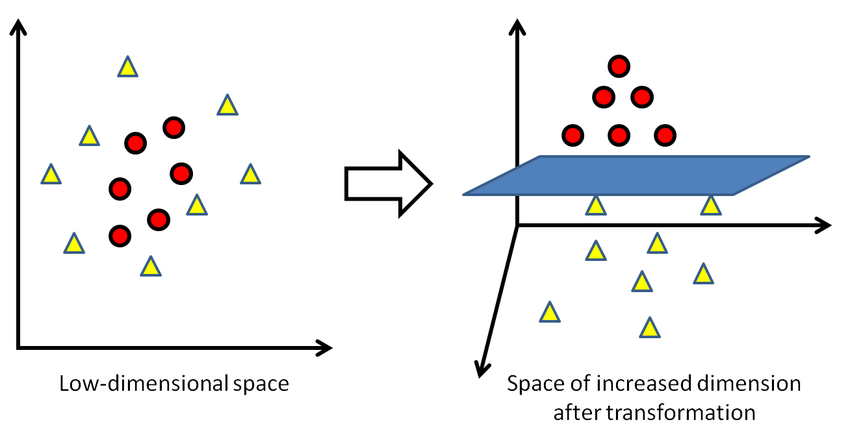
The choice of the kernel depends on the dataset. Popular kernels include:

Gaussian kernel
sigmoid kernel
polynomial kernel
radial basis function

Frameworks

scikit-learn provides utilities for SVMs in Python. Let’s look at a simple example.

We start by creating some dummy data.

import matplotlib.pyplot as plt
import numpy as np

# Fancy plots
plt.style.use("ggplot")

# Seed to reproduce experiment
np.random.seed = 1969

# 50 data points from each class
n = 50

# Class 1
X0 = np.random.randn(n)
Y0 = X0 * 2.0 + 3.0
Y0 += np.random.randn(n) # add noise

# Class 2
X1 = np.random.randn(n)
Y1 = X1 * 1.7 + 6.0
Y1 += np.random.randn(n) # add noise

class1 = np.vstack((X0, Y0)).T
class2 = np.vstack((X1, Y1)).T

data_points = np.vstack((class1, class2))
labels = np.concatenate((np.zeros(n), np.ones(n)))

plt.scatter(X0, Y0, alpha=0.75)
plt.scatter(X1, Y1, alpha=0.75)

plt.show()

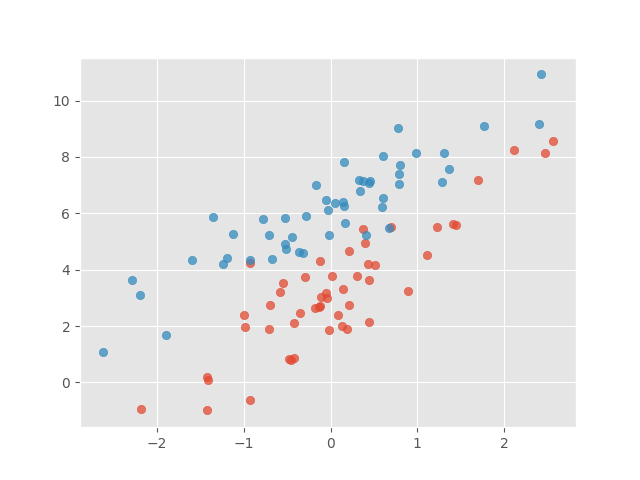
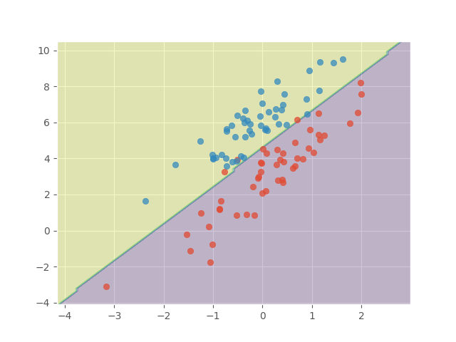
Next, we use the provided SVM tools from scikit-learn to fit the best linear separater.

from sklearn import svm
from sklearn.inspection import DecisionBoundaryDisplay

model = svm.SVC(kernel="linear")
model = model.fit(data_points, labels)

disp = DecisionBoundaryDisplay.from_estimator(
    model,
    data_points,
    response_method="predict",
    alpha=0.25,
)

plt.scatter(X0, Y0, alpha=0.75)
plt.scatter(X1, Y1, alpha=0.75)

plt.show()

Are SVMs outdated?

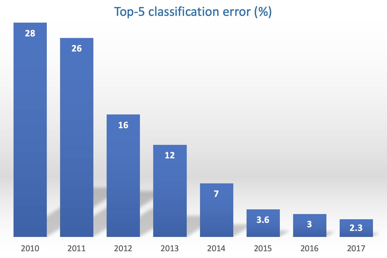
The figure above shows the improvement of image classification models over time on the ImageNet dataset. SVMs were state-of-the-art for image classification until the publication of AlexNet in 2012, which paved way for convolutional neural networks (CNNs) such as ResNet. Since 2017, state-of-the-art models have moved to transformers (like Google’s BERT and OpenAI’s GPT).

Interestingly, the architecture for AlexNet is very similar to LeNet (1998) and neural network concepts existed in the 1980s. However, they only took off decades later due to advancements in hardware and availability of large datasets, which are crucial for neural networks to perform well.

From this, we can make 2 arguments:

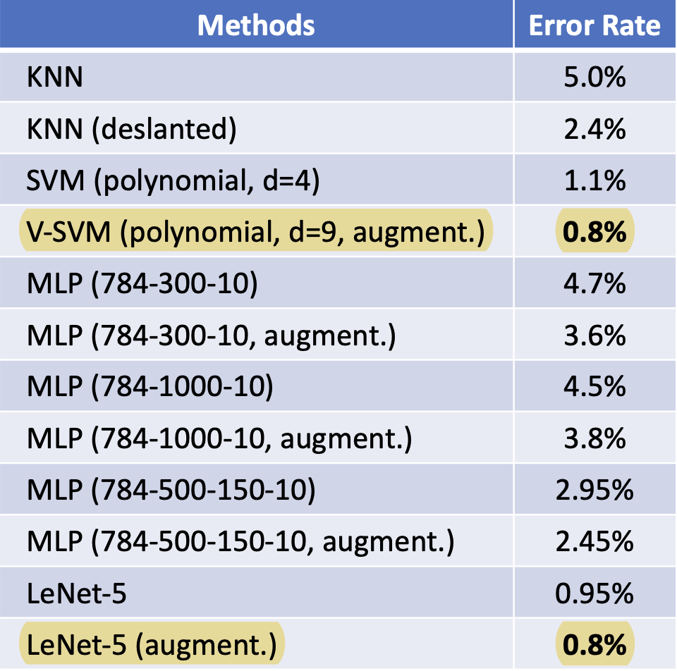
The newer state-of-the-art architectures like CNNs and transformers have millions (even billions) of tunable parameters. For simple tasks like digit handwriting recognition, SVMs perform well (see stats below) and offer a much cheaper solution to CNNs and transformers.
With rapid technology advancements in many fields, SVMs have potential to once again become state-of-the-art in the future.

Support Vector Machines

Motivation

Binary linear classifier

Initial steps

Extending to higher dimensions

Formulating the problem

Training the model: Gradient descent

Generalisations and extensions

Multi-class classification

Kernel trick

Frameworks

Are SVMs outdated?

Further reading

More Blog Posts