The Intuition behind Convolutional Neural Networks
Mar 28, 2024
Freddy
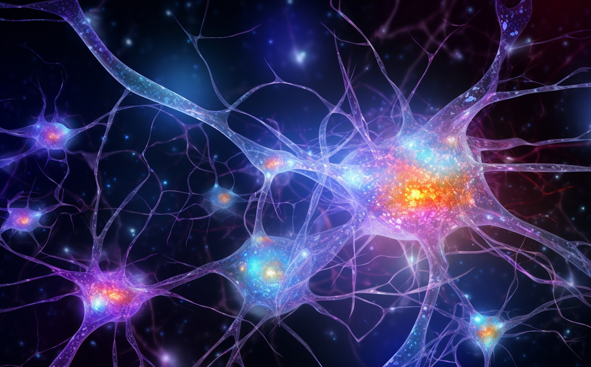
Before convolutional neural networks became popular, neural networks would often struggle with 2D data like image classification and image segmentation. In this article, we’ll dive into a bit of history to uncover the motivation behind convolutional neural networks, then understand the idea behind how and why they work.
Motivating Background
The core of all problems can be described as a mapping from an input space to an output space, and our goal is to solve this mapping (or approximate it as best as we can in practical settings), whether it be via machine learning or other methods.
For example, image classification involves mapping an image to a class label, while image segmentation involves mapping an image to a pixel-wise mask (that is, an image to another image).
Before convolutional neural networks (CNNs) became mainstream, neural networks often consisted of fully-connected (FC) layers. The building block of an FC layer can be described as a linear layer followed by an activation function.
A linear layer with a non-linear activation function is a universal approximator. This means given any input, the weights \({W}\) and bias \({b}\) can be chosen such that the ouput \({\hat{y}}\) is very close to the true output \({y}\).
Let’s consider a binary image segmentation task: given an image, identify the cat. A naive approach would be to take each pixel colour value and concatenate them into a 1D vector. Then, apply a linear layer with sigmoid activation to output another 1D vector of the same shape, which can be unfolded to represent the segmented output. However, there are 2 major problems:
- Neighbouring pixels are related to each other. By concatenating the image, we are losing spatial information.
- The network only learns a global approximation to the current input image. It does not generalise well to new images.
The 2nd problem is known as high bias, and it is demonstrated below. Say our network performs well on the training image.
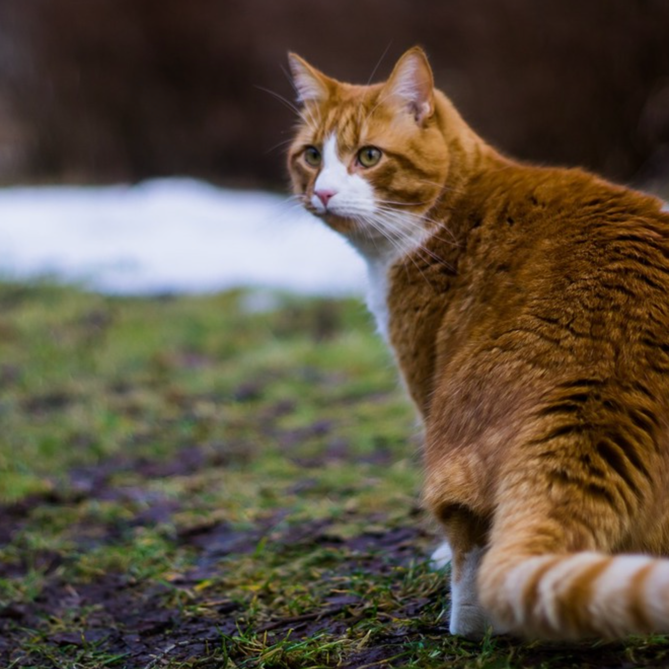
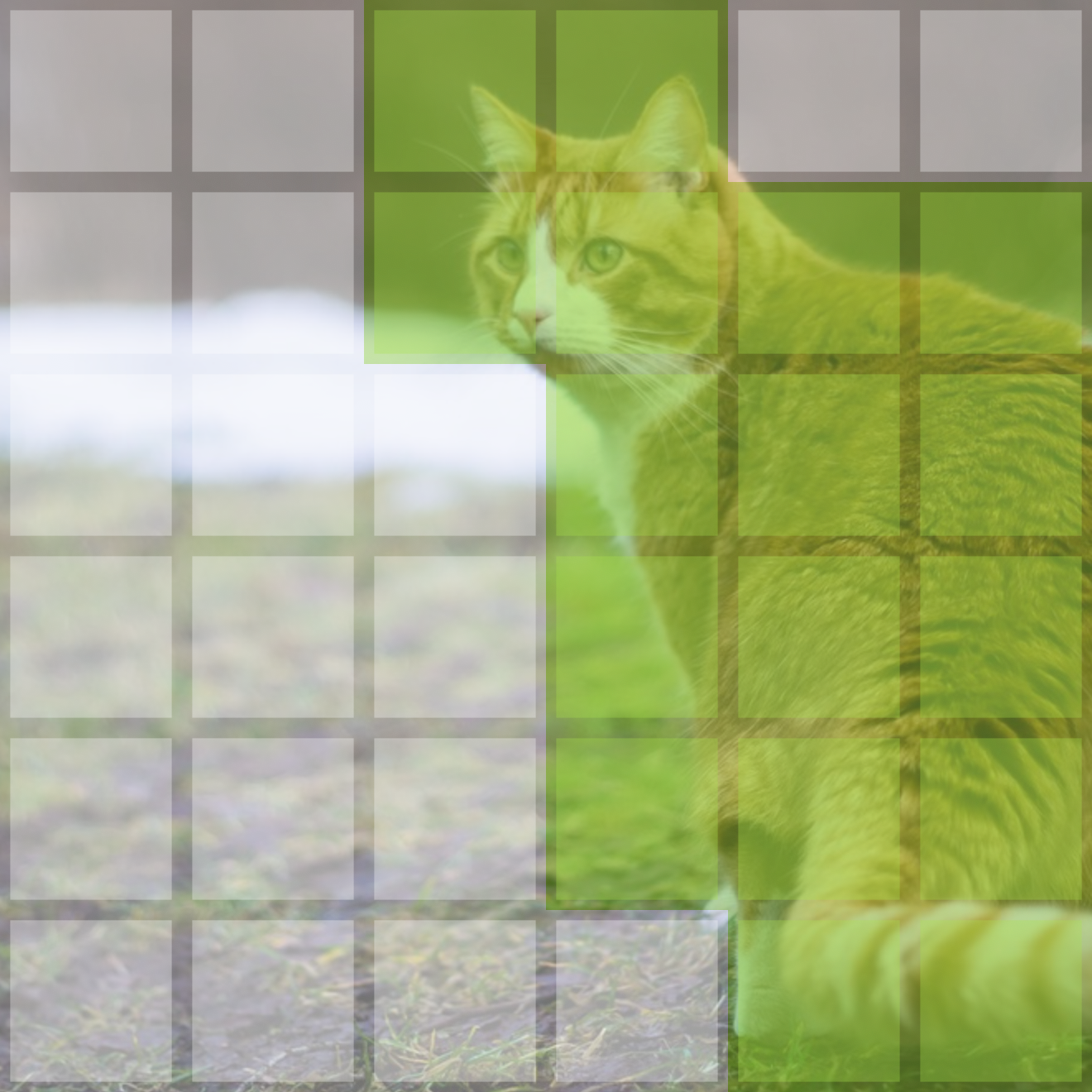
However, our 1-layer network is very rigid. Due to the bias-variance tradeoff, it has very low variance and generates a similar mask for the test image, incorrectly segmenting it.
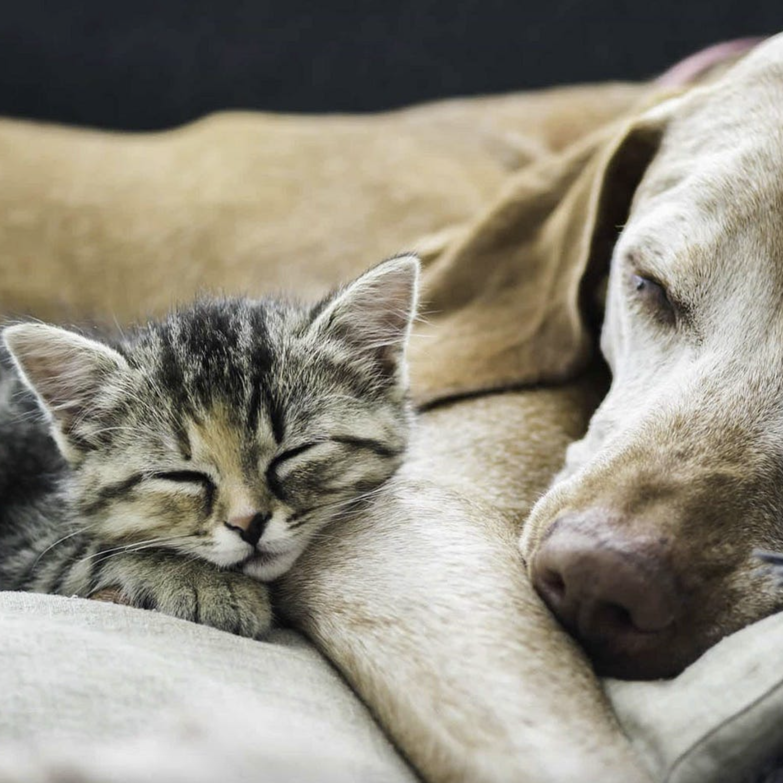
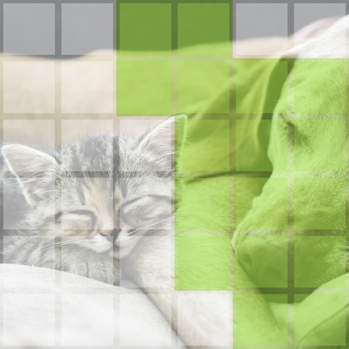
In this case, even though we are using a global approximator, it is not good enough - we’d have to retrain the network every time we encounter a new image. More generalisable models involve deeper layers to capture local patterns, but stacking FC layers on top of each other result in a large number of parameters which is infeasible for imaging tasks. Plus, spatial information is still not being leveraged.
This motivates the need for CNNs. In this post, we will focus on CNNs for 2D data, like images.
Convolutional Neural Networks
In essence, what we’ve previously done was to look at the entire image at once in 1 FC layer. The idea behind CNNs is to shrink this window down and look at patches of the image at a time.
Since each neuron now only has access to its corresponding patch, it is forced to learn local patterns. We continue to add more layers, increasing its receptive field so that the neurons in deeper layers can learn global patterns while preserving spatial invariance.
Let’s dive into the details.
Convolution
Previously, we mentioned linear regression: \({z = Wx + b}\) where \({x}\) is the values of the input image pixels and \({W}\) is the weights. For example, let our image have dimensions 6x6.
\[\begin{bmatrix} 0 & 0 & 0 & 255 & 255 & 0 \\ 0 & 0 & 0 & 255 & 255 & 0 \\ 127 & 127 & 127 & 255 & 255 & 127 \\ 127 & 127 & 127 & 255 & 255 & 127 \\ 0 & 0 & 0 & 255 & 255 & 0 \\ 0 & 0 & 0 & 127 & 127 & 0 \end{bmatrix}\]If \({z}\) is a scalar, then for our concatenated vector \({x}\) of size 36, \({W}\) would also have size 36, and we essentially calculate the dot product of \({W}\) and \({x}\).
The same concept applies to convolutions! However, instead of \({W}\) matching the size of \({x}\), we use a smaller filter, for example, a 3x3 filter. We refer to this as the kernel.
\[\begin{bmatrix} -1 & 0 & 1 \\ -2 & 0 & 2 \\ -1 & 0 & 1 \end{bmatrix}\]Of course, now we can’t perform dot product over the entire image \({x}\), but we can perform it over a patch. We start on the top right.
Note: I’m abusing notation a bit here, but if you think of these as dot products, treat them as vectors of size 9. However, convolutions are performed with the inputs as matrices.
\[\begin{bmatrix} 0 & 0 & 0 \\ 0 & 0 & 0 \\ 127 & 127 & 127 \end{bmatrix} \cdot \begin{bmatrix} -1 & 0 & 2 \\ -2 & 0 & 4 \\ -1 & 0 & 2 \end{bmatrix} = 127 \times -1 + 127 \times 2 = 127\]Now, we slide the filter to the right by 1 pixel.
\[\begin{bmatrix} 0 & 0 & 255 \\ 0 & 0 & 255 \\ 127 & 127 & 255 \end{bmatrix} \cdot \begin{bmatrix} -1 & 0 & 2 \\ -2 & 0 & 4 \\ -1 & 0 & 2 \end{bmatrix} = 1913\]We repeat this for each patch, and we get an output. We have performed a convolution operator and is denoted as \({\ast}\).
\[\begin{bmatrix} 0 & 0 & 0 & 255 & 255 & 0 \\ 0 & 0 & 0 & 255 & 255 & 0 \\ 127 & 127 & 127 & 255 & 255 & 127 \\ 127 & 127 & 127 & 255 & 255 & 127 \\ 0 & 0 & 0 & 255 & 255 & 0 \\ 0 & 0 & 0 & 127 & 127 & 0 \end{bmatrix} \ast \begin{bmatrix} -1 & 0 & 2 \\ -2 & 0 & 4 \\ -1 & 0 & 2 \\ \end{bmatrix} = \begin{bmatrix} 127 & 1913 & 1913 & -766 \\ 381 & 1659 & 1659 & -258 \\ 381 & 1659 & 1659 & -258 \\ 127 & 1657 & 1657 & -638 \end{bmatrix}\]This is what it looks like in action.
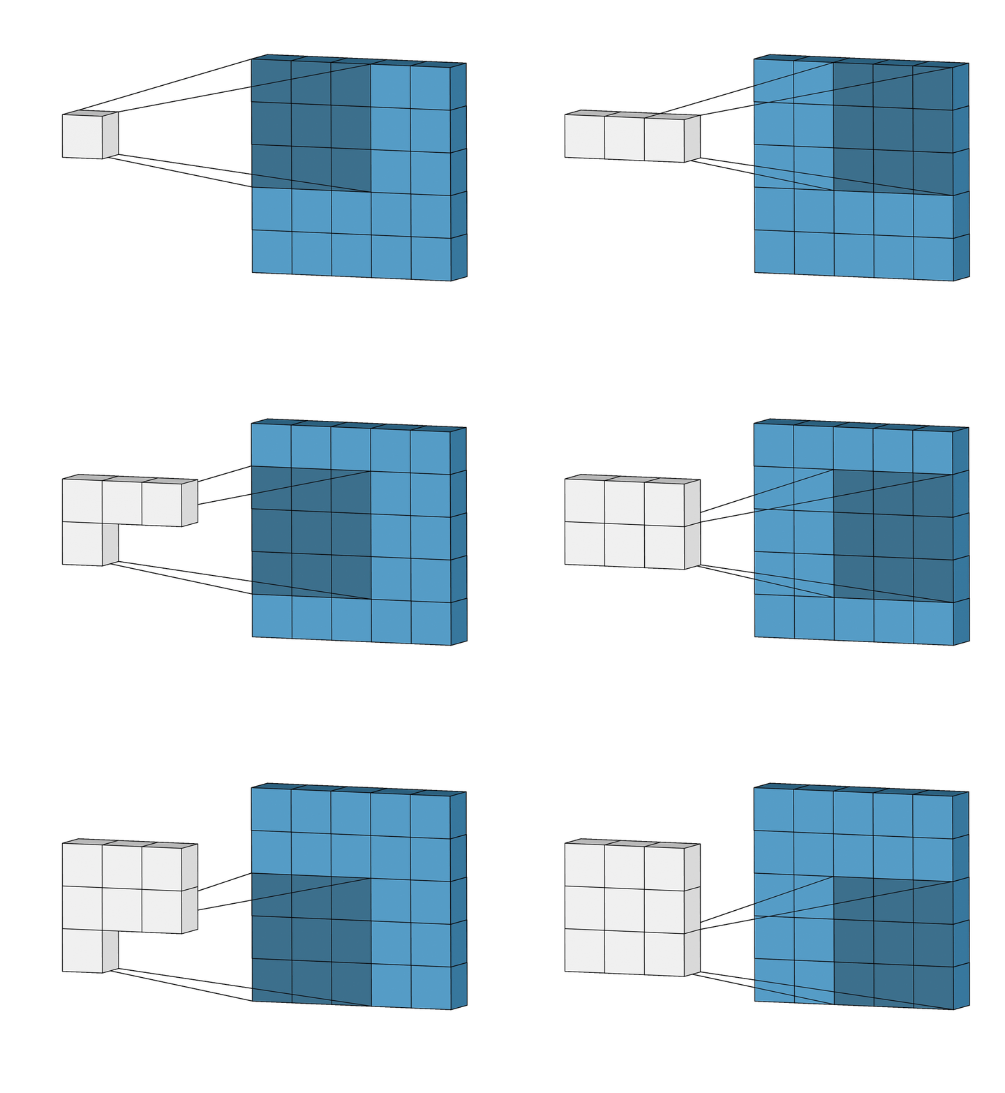
A key observation is that we are reusing the kernel for each patch, so the number of weights in our model remains small and manageable.
Now, we have a 4x4 output. This is known as a feature map. Each cell in the feature map is a neuron with a receptive field of 3x3. That is, its value is dependent on a 3x3 patch of the original input image.
Here, the ReLU activation is commonly used, as it can be interpreted as a gate: if the value is negative, it prevents gradient flow during backprop (the stage where the model weights get updated and the network learns), thus the neuron gets switched off. This is useful for controlling which areas of the image the deeper layers focus on - a bit like attention.
Let’s perform another convolution on the feature map with a different kernel.
\[\begin{bmatrix} 127 & 1913 & 1913 & -766 \\ 381 & 1659 & 1659 & -258 \\ 381 & 1659 & 1659 & -258 \\ 127 & 1657 & 1657 & -638 \end{bmatrix} \ast \begin{bmatrix} 1 & 1 & 1 \\ 1 & -8 & 1 \\ 1 & 1 & 1 \end{bmatrix} = \begin{bmatrix} -3580 & -5751 \\ -4092 & -6135 \end{bmatrix}\]Now, we have another feature map. Each neuron has a receptive field of 5x5, so its vision is almost the entire 6x6 image! This allows the neurons in this 2nd layer to learn global patterns that build upon the local patterns learned in the previous layer.
Towards the end of the convolutional network, we would sometimes flatten the feature map into a 1D vector and pass it through an FC layer with an activation function (like we did in our initial approach).
\[\sigma \left( \begin{bmatrix} -3580 & -5751 & -4092 & -6135 \end{bmatrix} \cdot \begin{bmatrix} 1 & 1 & -1 & -1 \end{bmatrix} \right) = 1\]Designing ConvNet Architecture in Practice
In practice, for each layer, we’d have multiple kernels instead of just 1. For example, if we have 32 kernels in the first layer (applying each kernel like how we did above), we’d have 32 feature maps. The weights for each kernel are different, so each feature map captures different patterns.
Then, instead of flattening the 2x2 feature map like we did, we would flatten a 2x2x32 tensor to pass into the FC layer.
To interpret this, think of our cat segmentation task. Here it is again.

To identify a cat, it’s easier to break this down into subtasks: 1 channel is responsible for detecting the pointy ears, another channel to detect the tail, and so on. Each channel’s responsibility can be more abstract: edge detection, gradient contour, etc.
Finally, we aggregate all of our information on the subtasks (i.e. flattening all feature maps) to predict the output. For segmentation in particular, we would use transposed convolutions to upscale the feature maps back to the original image. This is not covered in this post, but the intuition is the same.
Further Reading
This article covers the motivation behind CNNs and the intuition behind convolution operators and how CNNs work.
In practice, the architecture is delicate and many other techniques are applied to ensure the network trains well and generalises to unseen data. These include:
- Pooling to accelerate the growth of receptive fields and decrease in feature map size.
- Batch Normalisation - note how in our example calculations, the values get very large very quickly. Normalising the values after each layer helps with model stability.
- ResNet is a state-of-the-art architecture that introduces skip connections to enable gradient flow. This allows very deep networks (hundreds of layers) to train well and perform in complex tasks like classifying an image into 1000 classes.
- Data augmentation, dropout and other techniques to prevent overfitting.
More Blog Posts
The Intuition behind Convolutional Neural Networks
The UCI Protocol for Chess Engines
Setting Up Unrestricted ChatGPT Locally on Mac
Histogram Equalisation for Colour Images
Enhancing Greyscale Image Contrast through Histogram Equalisation
On the Philosophy and Design Choices of this Site
Benchmarking Loops in JavaScript
Looping Through a List in JavaScript